Euler Examples

Search

Benford's Law

It is a well known fact and it has been observed in many real life data that the first digit of the data is not distributed evenly among all possible first digits 1 to 9. Rather the observed distribution for the digit i is

This is called Benford's law.

To test this law, I stole stock data from an site, and listed the daily trade volume of their stock into a file.

>v=readmatrix("volumes.dat")';

Here are the first 100 values.

>v[1:200]

[544157,  544157,  156075,  11862,  265267,  1.71407e+006,  479429,
1.68337e+006,  22709,  130265,  42516,  41107,  6995,  149473,
191975,  62920,  42462,  39557,  63524,  16511,  865995,  48299,
69100,  109735,  86305,  84685,  237742,  122700,  153005,  137054,
73998,  18846,  55636,  68715,  23939,  16670,  149444,  129363,
290037,  6582,  187479,  8488,  26133,  81853,  26185,  25048,  80988,
213087,  881591,  3.18527e+006,  117500,  86400,  113609,  18719,
1.05462e+006,  1.77765e+007,  1.71189e+007,  650646,  1.47722e+006,
270910,  456247,  67000,  355126,  489772,  916030,  1859,  95172,
118442,  125030,  172168,  101264,  265043,  93265,  588767,
3.66473e+006,  2.10848e+006,  147272,  452850,  2.51024e+006,  129672,
599131,  1.17062e+006,  43360,  3.53408e+006,  2.15011e+006,  261405,
10500,  41615,  1.01669e+006,  127458,  226756,  101700,  2.7435e+006,
274591,  291125,  14340,  59780,  178830,  1.21082e+006,  128018,
856704,  378086,  664557,  405999,  828502,  335948,  576086,  604670,
134000,  83000,  654082,  812007,  639507,  3.24893e+006,  268568,
3.93623e+006,  9.15216e+006,  8.02835e+006,  1.8367e+006,  221005,
386657,  1.57159e+006,  68764,  58385,  896267,  30670,  5.0522e+006,
93478,  3.66215e+006,  279015,  5650,  726680,  136385,  106236,
490220,  304752,  1.52216e+006,  1.95674e+006,  1.97216e+006,
 ... ]

To find the first digit of a number in its decimal representation, we can use the following function.

>function fd(x) ...
 n=floor(log10(x));
 return floor(x/10^n)
 endfunction

The expected distribution is the following.

>d=log10(2:10)-log10(1:9)

[0.30103,  0.176091,  0.124939,  0.09691,  0.0791812,  0.0669468,
0.0579919,  0.0511525,  0.0457575]

Let us plot the distribution of the first digits in our data versus the expected distribution.

>columnsplot(getmultiplicities(1:9,fd(v))/length(v));  ...
   plot2d(1:9,d,>add);  ...
   plot2d(1:9,d,>points,>add); ...
   insimg;

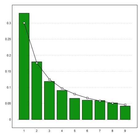
It is obvious that Benford's law is a better description of the reality than the assumption of an equal distribution.

Let us perform a statistical test to check the distribution. We first need the frequencies of the first digits in v.

>frequ=count(fd(v)-1,9)

[976,  530,  350,  267,  195,  178,  175,  152,  124]

With an equal distribution, we expect about 327 cases for each digit.

>nf=sum(frequ), fe=nf/9

2947
327.444444444

The chi-square test fails, of course.

>chitest(frequ,ones(1,9)*fe)

0

However, the chi-test fails also for our expected distribution, though not as badly as before.

>chitest(frequ,d*nf)

0.00887027918168

One could argue, that the distribution of the values is exponential. But this is not really the case. A logarithmic distribution of the random variable X would satisfy

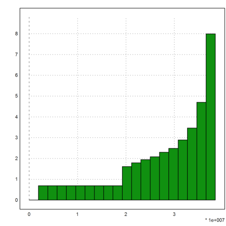
If we compute the logarithms for a cumulative frequency count of the values y, we see, that it is by no means linear.

>{x,y}=histo(v,20); plot2d(x,log(cumsum(flipx(y))),bar=true):

Let us compare this with an exponential distribution with the same mean value.

>m=mean(v)

469396.739396

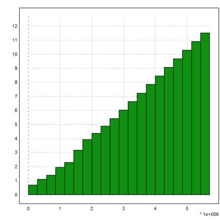
The following Monte Carlo simulation produces such a distribution.

>vt=-log(random(1,100000))*m; mean(vt)

467459.444843

>{x,y}=histo(vt,20); plot2d(x,log(cumsum(flipx(y))),>bar):

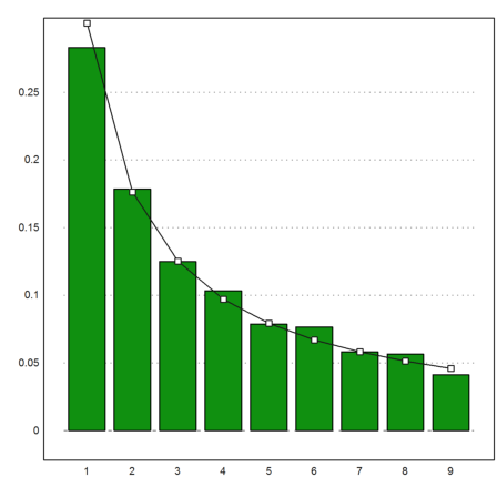
Let us compare the distributing of the first digits we found in our sample with an exponential distribution. For this, we produce a sequence of first digits, which are distributed according to Benford's law.

>va=fd(10^random(1,nf));

We insert these into the same plot as above.

>columnsplot(getmultiplicities(1:9,fd(va))/length(va));  ...
   plot2d(1:9,d,>add);  ...
   plot2d(1:9,d,>points,>add); ...
   insimg;

>frequa=count(fd(va)-1,9)

[834,  526,  368,  304,  232,  225,  171,  166,  121]

Most likely, the chi-square test cannot reject the distribution d for our Monte Carlo data.

>chitest(frequa,d*nf)

0.183718883574

A more general way to express Benford's law is to state that the fractions of the decadic logarithm of the data is distributed evenly in [0,1].

We can plot the distribution of these fractions for our data.

>plot2d(mod(log10(v),1),>distribution):

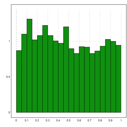
The result looks very good.

Examples